prove cbrt in CORE-MATH

原文：Correctly Rounded Cubic Root Evaluation in Double Precision — Alexei Sibidanov, Paul Zimmermann（CORE-MATH 项目）。

本文为中英双语对照翻译，并收录了原文的全部插图（图 3–5 原为四幅子图，此处按原文 2×2 版式拼合为一图）；原文由 OCR 得到，其中明显的讹误（包括公式编号）已在翻译时径直修正。

EN

The cubic root $x=\sqrt[3]{a}$ is a real root of an algebraic equation:

$$\begin{array}{}\text{(1)}& f(x)=x^3-a=0.\end{array}$$

There is a closed form solution for Eq. (1) but it already requires the cubic root function so other methods have to be employed e.g. Newton iteration.

中

立方根 $x=\sqrt[3]{a}$ 是如下代数方程的一个实根：

$$\begin{array}{}\text{(1)}& f(x)=x^3-a=0.\end{array}$$

式 (1) 虽然有闭式解，但求解过程本身就要用到立方根函数，因此必须采用其他方法，例如 Newton 迭代。

EN

Let $x_0$ be an initial approximation of the cubic root then

$$\begin{array}{}\text{(2)}& h_0=f(x_0)/a=(x_0^3-a)/a=(x_0^3-a)r_a\end{array}$$

is the relative error of Eq. (1) with respect to $a$ and $r_a=1/a$ is the reciprocal of $a$. The next better approximation $x_1$ can be derived as

$$\begin{array}{}\text{(3)}& x_1=x_0-\frac{1}{3}{x}_0{h}_0\end{array}$$

with about two times more significant figures than in $x_0$. This procedure should be repeated until it reaches required precision.

中

设 $x_0$ 是立方根的一个初始近似，那么

$$\begin{array}{}\text{(2)}& h_0=f(x_0)/a=(x_0^3-a)/a=(x_0^3-a)r_a\end{array}$$

就是式 (1) 相对于 $a$ 的相对误差，其中 $r_a=1/a$ 是 $a$ 的倒数。下一个更好的近似 $x_1$ 可由下式导出：

$$\begin{array}{}\text{(3)}& x_1=x_0-\frac{1}{3}{x}_0{h}_0\end{array}$$

其有效数字大约是 $x_0$ 的两倍。重复这一过程，直到达到所需精度。

EN

The generalization of the Newton iteration method to higher orders gives the following rule:

$$\begin{array}{}\text{(4)}& x_{i+1}=x_i(1-\frac{1}{3}{h}_i+\frac{2}{9}{h}_i^2-\frac{14}{81}{h}_i^3+\frac{35}{243}{h}_i^4-\frac{91}{729}{h}_i^5+\frac{728}{6561}{h}_i^6-\frac{1976}{19683}{h}_i^7+\frac{5434}{59049}{h}_i^8-\dots )\end{array}$$

where each additional term reduces the error of the next approximation $x_{i+1}$ by $h$. The coefficients of the polynomial expression in Eq. (4) are given by the series expansion of

$$\begin{array}{}\text{(5)}& \frac{1}{\sqrt[3]{1+h}}=\sum _{j=0}^{\mathrm{\infty }}{c}_j{h}^j.\end{array}$$

中

把 Newton 迭代法推广到更高阶，可得如下迭代规则：

$$\begin{array}{}\text{(4)}& x_{i+1}=x_i(1-\frac{1}{3}{h}_i+\frac{2}{9}{h}_i^2-\frac{14}{81}{h}_i^3+\frac{35}{243}{h}_i^4-\frac{91}{729}{h}_i^5+\frac{728}{6561}{h}_i^6-\frac{1976}{19683}{h}_i^7+\frac{5434}{59049}{h}_i^8-\dots )\end{array}$$

其中每增加一项，下一次近似 $x_{i+1}$ 的误差就降低一个 $h$ 的因子。式 (4) 中多项式表达式的系数由下式的级数展开给出：

$$\begin{array}{}\text{(5)}& \frac{1}{\sqrt[3]{1+h}}=\sum _{j=0}^{\mathrm{\infty }}{c}_j{h}^j.\end{array}$$

EN

Since $a$ and $x$ are represented as IEEE-754 double precision floating point numbers aka binary64 we can reduce exactly the input argument $a$ to the $[1,8]$ range to get $x\in [1,2]$ range and then scale it accordingly to get the final result. The binary scaling is a cheap and exact operation in the binary64 format and particularly for the cubic root without the danger of the overflow or underflow since the limited exponent range of the final result. The argument $a$ can be further reduced to the $[1,2]$ range but the result has to be scaled by $2^{n/3}$ before the final refinement to get the correctly rounded result since the values of $2^{n/3}$ with $n=1,2$ are inexact in the binary64 format.

中

由于 $a$ 和 $x$ 都表示为 IEEE-754 双精度浮点数（即 binary64），我们可以把输入参数 $a$ 精确地归约到 $[1,8]$ 区间，从而得到 $x\in [1,2]$，再相应地缩放得到最终结果。在 binary64 格式中，二进制缩放是一种廉价且精确的操作，对立方根尤其如此——由于最终结果的指数范围有限，不会有上溢或下溢的风险。参数 $a$ 还可以进一步归约到 $[1,2]$ 区间，但为了得到正确舍入的结果，在最后的精化之前必须用 $2^{n/3}$ 对结果进行缩放，因为当 $n=1,2$ 时 $2^{n/3}$ 的值在 binary64 格式中是不精确的。

EN

For arguments in the range [1, 2] Newton iterations for the cubic root always converges with the initial approximation $x_0=1.104$ in all orders in our tests. An example is shown in Fig. 1 for the high order given in Eq. (4). It shows that with a moderately precise initial approximation Newton iterations converge rapidly. For fast evaluation the initial approximation can be selected as a low order polynomial.

中

在我们的测试中，对于 [1, 2] 区间内的参数，取初始近似 $x_0=1.104$ 时，各阶立方根 Newton 迭代总是收敛的。图 1 给出了一个以式 (4) 的高阶迭代为例的示例。它表明，只要初始近似具有适当的精度，Newton 迭代就会迅速收敛。为了快速求值，初始近似可以选为一个低阶多项式。

EN

The error $h_0$ of the minimax approximations of the cubic root function by the second, third, fourth and fifth order polynomials is shown in Fig. 2. The error $h_1$ after the first step is shown in Fig. 3 for the second order Newton iteration, Fig. 4 for the third order, and Fig. 5 for the quartic order. These calculations are performed in the binary64 format so the limited precision of the format is immediately seen even after the first high order iteration. So itself the cubic root calculated by this method cannot be correctly rounded due to intermediate rounding errors. The final refinement step using a compensated algorithm is needed.

中

用二阶、三阶、四阶和五阶多项式对立方根函数做 minimax 近似的误差 $h_0$ 如图 2 所示。第一步迭代之后的误差 $h_1$ 如图 3（二阶 Newton 迭代）、图 4（三阶）和图 5（四阶）所示。这些计算都在 binary64 格式中进行，因此即使在第一次高阶迭代之后，也能立刻看到格式有限精度的影响。所以，由于中间舍入误差的存在，用这种方法本身计算出的立方根无法做到正确舍入，还需要使用补偿算法的最终精化步骤。

EN

The final step has to be as simple as possible so it is the second order Newton iteration (Eq. (2) and (3)) where intermediate values are represented as an unevaluated sum of two binary64 numbers so the internal precision should be about 100 bits which largely exceeds the target precision of the result of 53 bits in binary64.

中

最后一步应当尽可能简单，因此选用二阶 Newton 迭代（式 (2) 和式 (3)），其中间值表示为两个 binary64 数的未求和（unevaluated sum），这样内部精度约为 100 位，远超 binary64 中 53 位的目标结果精度。

EN

The precision of the result before the final step should not hit the binary64 precision limit it should be just good enough that after the refinement—which doubles the number of significant figures—an additional refinement has to be done only in very rare cases when the rounding test fails. Based on this consideration and performance tests we select the initial cubic polynomial approximation and the third order Newton iteration step, see the top-right plots in Fig. 2 and 4.

中

最终步骤之前结果的精度不应触及 binary64 的精度上限，它只需足够好，使得经过精化（精化会使有效数字翻倍）之后，只有在舍入测试失败的极少数情况下才需要再做一次额外的精化。基于这一考虑以及性能测试，我们选择三次多项式初始近似加三阶 Newton 迭代步骤，见图 2 和图 4 右上角的子图。

EN

After the refinement with the compensated algorithm, the cubic root value is represented as an unevaluated sum $a+b$ of two binary64 numbers, where $e_a\ge e_b$ (i.e., the exponent of $a$ is larger or equal to that of $b$). We then apply the Fast2Sum algorithm to compute $x_2^{\mathrm{high}}=\circ (a+b)$, $z=\circ (x_2^{\mathrm{high}}-a)$, $x_2^{\mathrm{low}}=\circ (b-z)$, where $\circ ()$ denotes the current rounding mode.

中

经过补偿算法的精化之后，立方根的值表示为两个 binary64 数的未求和 $a+b$，其中 $e_a\ge e_b$（即 $a$ 的指数大于或等于 $b$ 的指数）。然后我们用 Fast2Sum 算法计算 $x_2^{\mathrm{high}}=\circ (a+b)$、$z=\circ (x_2^{\mathrm{high}}-a)$、$x_2^{\mathrm{low}}=\circ (b-z)$，其中 $\circ ()$ 表示当前的舍入模式。

Lemma 1

EN

Lemma 1. Whatever the rounding mode, we have $|x_2^{\mathrm{low}}|<2^{-52}$.

Proof. For rounding to nearest, this is a direct consequence of the Fast2Sum algorithm, since in that case we have $a+b=x_2^{\mathrm{high}}+x_2^{\mathrm{low}}$ exactly, and since $x_2^{\mathrm{high}}$ is the rounding to nearest of $a+b$, we have $|x_2^{\mathrm{low}}|\le \frac{1}{2}\mathrm{ulp}(x_2^{\mathrm{high}})$. For directed rounding, according to [1, Theorem 3.1], $x_2^{\mathrm{low}}$ is a faithful rounding of the error in the FP addition $x_2^{\mathrm{high}}=\circ (a+b)$. Let $\epsilon =(a+b)-x_2^{\mathrm{high}}$ be that error. Since $1\le a+b\le 2$, and $x_2^{\mathrm{high}}$ is a directed rounding of $a+b$, we have $|\epsilon |<\mathrm{ulp}(1)=2^{-52}$, thus a faithful rounding of that error cannot exceed $2^{-52}$. Now if a faithful rounding of $\epsilon$ is $\pm 2^{-52}$, this implies $|\epsilon |>2^{-52}+2^{-105}$, since $2^{-52}+2^{-105}$ is representable in binary64. This in turn implies $\mathrm{ulp}(b)<2^{-105}$, otherwise $a+b$ would be an integer multiple of $2^{-105}$, which would contradict $2^{-52}+2^{-105}<|\epsilon |<2^{-52}$. But since $|b|<2^{53}\mathrm{ulp}(b)$ this yields $|b|<2^{-52}$. In the Fast2Sum algorithm, when $x_2^{\mathrm{high}}=\circ (a+b)$ is rounded towards $a$, we get $z=0$ and $x_2^{\mathrm{low}}=b$, thus $|x_2^{\mathrm{low}}|<2^{-52}$. If $x_2^{\mathrm{high}}=\circ (a+b)$ is rounded away from $a$, say upwards if $b>0$, then $z=2^{-52}$, and since $x_2^{\mathrm{low}}=\circ (b-z)$ is rounded in the same direction, we get $x_2^{\mathrm{low}}>-z$. The same reasoning when rounding downwards for $b<0$ also gives $|x_2^{\mathrm{low}}|<2^{-52}$. □

中

引理 1. 无论舍入模式如何，都有 $|x_2^{\mathrm{low}}|<2^{-52}$。

证明。 对于就近舍入，这是 Fast2Sum 算法的直接推论：此时 $a+b=x_2^{\mathrm{high}}+x_2^{\mathrm{low}}$ 精确成立，又因为 $x_2^{\mathrm{high}}$ 是 $a+b$ 的就近舍入，所以 $|x_2^{\mathrm{low}}|\le \frac{1}{2}\mathrm{ulp}(x_2^{\mathrm{high}})$。对于方向舍入，根据 [1, Theorem 3.1]，$x_2^{\mathrm{low}}$ 是浮点加法 $x_2^{\mathrm{high}}=\circ (a+b)$ 中误差的忠实舍入（faithful rounding）。设 $\epsilon =(a+b)-x_2^{\mathrm{high}}$ 为该误差。由于 $1\le a+b\le 2$，且 $x_2^{\mathrm{high}}$ 是 $a+b$ 的一个方向舍入，我们有 $|\epsilon |<\mathrm{ulp}(1)=2^{-52}$，因此该误差的忠实舍入不会超过 $2^{-52}$。假如 $\epsilon$ 的某个忠实舍入为 $\pm 2^{-52}$，则意味着 $|\epsilon |>2^{-52}+2^{-105}$，因为 $2^{-52}+2^{-105}$ 在 binary64 中可表示。而这又意味着 $\mathrm{ulp}(b)<2^{-105}$，否则 $a+b$ 将是 $2^{-105}$ 的整数倍，与 $2^{-52}+2^{-105}<|\epsilon |<2^{-52}$ 矛盾。但由 $|b|<2^{53}\mathrm{ulp}(b)$ 可得 $|b|<2^{-52}$。在 Fast2Sum 算法中，当 $x_2^{\mathrm{high}}=\circ (a+b)$ 向 $a$ 所在方向舍入时，有 $z=0$ 且 $x_2^{\mathrm{low}}=b$，于是 $|x_2^{\mathrm{low}}|<2^{-52}$。若 $x_2^{\mathrm{high}}=\circ (a+b)$ 向远离 $a$ 的方向舍入（例如当 $b>0$ 时向上舍入），则 $z=2^{-52}$，又因为 $x_2^{\mathrm{low}}=\circ (b-z)$ 朝同一方向舍入，可得 $x_2^{\mathrm{low}}>-z$；当 $b<0$ 时向下舍入的情形同理，同样得到 $|x_2^{\mathrm{low}}|<2^{-52}$。□

EN

According to Lemma 1, we thus get an approximation $x_2^{\mathrm{high}}+x_2^{\mathrm{low}}$ of the cubic root with $|x_2^{\mathrm{low}}|<2^{-52}$. The difference of this approximation with the exact cubic root value is shown in Fig. 6. The maximal found error is $-0\text{x}1.fe62ec338\text{p}-77\approx -1.32\times {10}^{-23}$ and it occurs near the upper bound of the range. Thus to perform the rounding test in the round-to-nearest mode we need to check that $||x_2^{\mathrm{low}}|-2^{-53}|>2^{-76}$ which means that $x_2^{\mathrm{high}}$ is a correctly rounded cubic root value in binary64. In the directional modes we need to check both borders $|x_2^{\mathrm{low}}|>2^{-76}$ and $||x_2^{\mathrm{low}}|-2^{-52}|>2^{-76}$ to be sure that $x_2^{\mathrm{high}}$ is correctly rounded. For safety the limit $2^{-76}$ is increased 2 times to $2^{-75}$. Considering this limit we can conclude that the probability to fail the test is about $2^{-75}/2^{-52}\sim {10}^{-7}$. There is a special case of exact cubic roots which will be described later.

中

根据引理 1，我们得到了对立方根的一个近似 $x_2^{\mathrm{high}}+x_2^{\mathrm{low}}$，满足 $|x_2^{\mathrm{low}}|<2^{-52}$。该近似与精确立方根值的差如图 6 所示。实测的最大误差为 $-0\text{x}1.fe62ec338\text{p}-77\approx -1.32\times {10}^{-23}$，出现在区间的上界附近。因此，为了在就近舍入模式下进行舍入测试，我们需要检查 $||x_2^{\mathrm{low}}|-2^{-53}|>2^{-76}$，这表示 $x_2^{\mathrm{high}}$ 是 binary64 中一个正确舍入的立方根值。在方向舍入模式下，我们需要同时检查两个边界 $|x_2^{\mathrm{low}}|>2^{-76}$ 和 $||x_2^{\mathrm{low}}|-2^{-52}|>2^{-76}$，才能确保 $x_2^{\mathrm{high}}$ 正确舍入。出于安全考虑，把界限 $2^{-76}$ 放大 2 倍到 $2^{-75}$。从这一界限可以推断，测试失败的概率约为 $2^{-75}/2^{-52}\sim {10}^{-7}$。还有一类特殊的精确立方根情形，将在后面描述。

EN

If the rounding test fails we perform an additional second order Newton iteration step starting from $x_2^{\mathrm{high}}$ which is known to be very close to the correctly rounded cubic root just might be 1 ulp off. The difference of $x_3^{\mathrm{high}}$ (again $x_3=x_3^{\mathrm{high}}+x_3^{\mathrm{low}}$) with the exact cubic root value is shown in Fig. 7, 8, 9, 10 when FPU is operating in various rounding modes. As it is seen the maximal visible error is about $2^{-102}$ on the limited number of arguments.

中

如果舍入测试失败，我们就以 $x_2^{\mathrm{high}}$ 为起点再执行一步二阶 Newton 迭代，已知该值离正确舍入的立方根非常近，最多可能相差 1 个 ulp。当 FPU 在各种舍入模式下运行时，$x_3^{\mathrm{high}}$（同样 $x_3=x_3^{\mathrm{high}}+x_3^{\mathrm{low}}$）与精确立方根值的差如图 7、8、9、10 所示。可以看出，在这些数量有限的参数上，最大的可见误差约为 $2^{-102}$。

EN

Unfortunately even the last refinement is not enough for the worst cases to provide the correct rounded results, fortunately there are only a few such cases so we can test arguments and return already precomputed correctly rounded values.

中

遗憾的是，即便做最后一次精化，对于最坏情形仍不足以给出正确舍入的结果；所幸这类情形只占极少数，因此我们可以对这些参数进行测试，并直接返回预先算好的正确舍入值。

EN

In the round-to-nearest mode the exact cases, when both $a$ and $x$ are representable in the binary64 format exactly, always pass the first rounding test and round to correct values. Unfortunately one also finds that the inexact flag is raised despite the exact roots due to the intermediate rounding errors. In the directed rounding modes both rounding tests fail for exact cubic roots and $x_3^{\mathrm{high}}$ can be 1 ulp off the correctly rounded value. Such cases have to be detected and the flag has to be restored to the state just before the function call.

中

在就近舍入模式下，当 $a$ 和 $x$ 都能在 binary64 格式中精确表示时（精确情形），它们总能通过第一次舍入测试并舍入到正确的值。遗憾的是，尽管根是精确的，由于中间舍入误差，inexact 标志仍会被置位。在方向舍入模式下，对于精确立方根，两次舍入测试都会失败，并且 $x_3^{\mathrm{high}}$ 可能偏离正确舍入值 1 个 ulp。这类情形必须被检测出来，并且标志位需要恢复到函数调用之前的状态。

EN

There are 104032 distinct binary64 numbers $x$ in the [1, 2] range which might be exact solutions of Eq. (1) with the one with largest numerator being $208063/2^{17}$, where $208063=\lfloor 2^{53/3}\rfloor$. Thus, for exact cubic roots, and rounding to nearest, at least 35 last bits of $x_2^{\mathrm{high}}$ have to be zero. For exact cubic roots with a directed rounding mode, the last 35 bits of $x_3^{\mathrm{high}}$ should be all 0 or 1 (note that the first rounding test will always fail in that case). The test of the last bits of x alone to detect the exact cases is not enough since there are cases when the cubic root of a has 35 zero bits but it is not an exact root. For example, when we have exact relation $x=\sqrt[3]{a}$ in binary64 then $\sqrt[3]{a\pm 1\mathrm{ulp}}$ would be also very close to $x$ and thus would inherit the property of the last 35 bits. So we also need to test that the difference between $x$ and its rounded-to-nearest value in binary64 is smaller than the smallest difference between the cubic root values of two consecutive binary64 values to detect exact cases.

中

在 [1, 2] 区间内，共有 104032 个不同的 binary64 数 $x$ 可能是式 (1) 的精确解，其中分子最大的是 $208063/2^{17}$，这里 $208063=\lfloor 2^{53/3}\rfloor$。因此，对于精确立方根，在就近舍入模式下，$x_2^{\mathrm{high}}$ 的最后至少 35 位必须为零；而在方向舍入模式下，$x_3^{\mathrm{high}}$ 的最后 35 位应当全为 0 或全为 1（注意此时第一次舍入测试总会失败）。仅仅检测 $x$ 的最后几位不足以识别精确情形，因为存在这样的情况：$a$ 的立方根末 35 位为零，但它并不是精确的根。例如，当 binary64 中存在精确关系 $x=\sqrt[3]{a}$ 时，$\sqrt[3]{a\pm 1\mathrm{ulp}}$ 也会非常接近 $x$，因而会继承末 35 位的这种性质。所以，为了识别精确情形，我们还需检测 $x$ 与其 binary64 就近舍入值之差，是否小于相邻两个 binary64 数立方根之间的最小差值。

Lemma 2

EN

Lemma 2. Let $a$ be a binary64 number such that $1\le a<8$, and $a^{1/3}$ is not exactly representable in binary64. Let $x$ be a binary64 number such that $x^3$ is also a binary64 number, and $x$ is closest to $a^{1/3}$ (in case of tie, any value is ok). Then the distance from $a^{1/3}$ to $x$ is at least $4.66\cdot {10}^{-17}$.

Proof. We first deal with the special cases where $a$ is a power of 2. First $a$ cannot be 1, since $1^{1/3}$ is exactly representable in binary64. If $a=2$, we get $x=165140/2^{17}$ and $|a^{1/3}-x|>2\cdot {10}^{-6}$. If $a=4$, we get $x=104032/2^{16}$, and $|a^{1/3}-x|>1\cdot {10}^{-6}$. Now assume that $a$ is not a power of 2. Since $x^3$ is a binary64 number, and $x^3\ne a$, we have $|x^3-a|\ge \mathrm{ulp}(a)$ (since $a$ is not a power of 2). Write $a^{1/3}=x+\epsilon$. Then $a=x^3+3x^2\epsilon +3x{\epsilon }^2+{\epsilon }^3$. Thus $|3x^2\epsilon +3x{\epsilon }^2+{\epsilon }^3|\ge \mathrm{ulp}(a)$. In the case where $1\le a<2$ we have $\mathrm{ulp}(a)=2^{-52}$, and writing $\delta =|\epsilon |$:

$$\delta \ge \frac{2^{-52}}{3x^2}-\frac{{\delta }^2}{x}-\frac{{\delta }^3}{3x^2},$$

where $x\le x_0=165141/2^{17}$. Thus

$$\delta \ge \frac{2^{-52}}{3x_0^2}-{\delta }^2-\frac{{\delta }^3}{3}.$$

The corresponding equation has a single real root ${\delta }_0\approx 4.66\cdot {10}^{-17}$, and for $\delta <{\delta }_0$, the above inequality does not hold. In the case where $2\le a<4$, we have $\mathrm{ulp}(a)=2^{-51}$, and writing $\delta =|\epsilon |$:

$$\delta \ge \frac{2^{-51}}{3x^2}-\frac{{\delta }^2}{x}-\frac{{\delta }^3}{3x^2},$$

where $x\le x_1=104032/2^{16}$. Thus

$$\delta \ge \frac{2^{-51}}{3x_1^2}-{\delta }^2-\frac{{\delta }^3}{3}.$$

The corresponding equation has a single real root ${\delta }_1\approx 5.87\cdot {10}^{-17}$, and for $\delta <{\delta }_1$, the above inequality does not hold. In the case where $4\le a<8$, we have $\mathrm{ulp}(a)=2^{-50}$, and writing $\delta =|\epsilon |$:

$$\delta \ge \frac{2^{-50}}{3x^2}-\frac{{\delta }^2}{x}-\frac{{\delta }^3}{3x^2},$$

where $x\le x_2=2$. Thus

$$\delta \ge \frac{2^{-50}}{3x_2^2}-{\delta }^2-\frac{{\delta }^3}{3}.$$

The corresponding equation has a single real root ${\delta }_2\approx 7.40\cdot {10}^{-17}$, and for $\delta <{\delta }_2$, the above inequality does not hold. In summary, for $|\epsilon |\le min({\delta }_0,{\delta }_1,{\delta }_2)$, the inequality does not hold, thus we have $|\epsilon |>min({\delta }_0,{\delta }_1,{\delta }_2)\ge 4.66\cdot {10}^{-17}$. □

中

引理 2. 设 $a$ 是一个 binary64 数，满足 $1\le a<8$，且 $a^{1/3}$ 在 binary64 中不能精确表示。设 $x$ 是一个 binary64 数，使得 $x^3$ 也是 binary64 数，且 $x$ 最接近 $a^{1/3}$（若等距，任取一个即可）。则从 $a^{1/3}$ 到 $x$ 的距离至少为 $4.66\cdot {10}^{-17}$。

证明。 我们先处理 $a$ 是 2 的幂的若干特殊情形。首先 $a$ 不能等于 1，因为 $1^{1/3}$ 在 binary64 中可以精确表示。若 $a=2$，则 $x=165140/2^{17}$，且 $|a^{1/3}-x|>2\cdot {10}^{-6}$。若 $a=4$，则 $x=104032/2^{16}$，且 $|a^{1/3}-x|>1\cdot {10}^{-6}$。接下来假设 $a$ 不是 2 的幂。由于 $x^3$ 是 binary64 数，且 $x^3\ne a$，我们有 $|x^3-a|\ge \mathrm{ulp}(a)$（因为 $a$ 不是 2 的幂）。记 $a^{1/3}=x+\epsilon$，则 $a=x^3+3x^2\epsilon +3x{\epsilon }^2+{\epsilon }^3$。因此 $|3x^2\epsilon +3x{\epsilon }^2+{\epsilon }^3|\ge \mathrm{ulp}(a)$。当 $1\le a<2$ 时，有 $\mathrm{ulp}(a)=2^{-52}$，记 $\delta =|\epsilon |$：

$$\delta \ge \frac{2^{-52}}{3x^2}-\frac{{\delta }^2}{x}-\frac{{\delta }^3}{3x^2},$$

其中 $x\le x_0=165141/2^{17}$。于是

$$\delta \ge \frac{2^{-52}}{3x_0^2}-{\delta }^2-\frac{{\delta }^3}{3}.$$

对应方程只有一个实根 ${\delta }_0\approx 4.66\cdot {10}^{-17}$，且当 $\delta <{\delta }_0$ 时上述不等式不成立。当 $2\le a<4$ 时，有 $\mathrm{ulp}(a)=2^{-51}$，记 $\delta =|\epsilon |$：

$$\delta \ge \frac{2^{-51}}{3x^2}-\frac{{\delta }^2}{x}-\frac{{\delta }^3}{3x^2},$$

其中 $x\le x_1=104032/2^{16}$。于是

$$\delta \ge \frac{2^{-51}}{3x_1^2}-{\delta }^2-\frac{{\delta }^3}{3}.$$

对应方程只有一个实根 ${\delta }_1\approx 5.87\cdot {10}^{-17}$，且当 $\delta <{\delta }_1$ 时上述不等式不成立。当 $4\le a<8$ 时，有 $\mathrm{ulp}(a)=2^{-50}$，记 $\delta =|\epsilon |$：

$$\delta \ge \frac{2^{-50}}{3x^2}-\frac{{\delta }^2}{x}-\frac{{\delta }^3}{3x^2},$$

其中 $x\le x_2=2$。于是

$$\delta \ge \frac{2^{-50}}{3x_2^2}-{\delta }^2-\frac{{\delta }^3}{3}.$$

对应方程只有一个实根 ${\delta }_2\approx 7.40\cdot {10}^{-17}$，且当 $\delta <{\delta }_2$ 时上述不等式不成立。综上，当 $|\epsilon |\le min({\delta }_0,{\delta }_1,{\delta }_2)$ 时不等式不成立，因此有 $|\epsilon |>min({\delta }_0,{\delta }_1,{\delta }_2)\ge 4.66\cdot {10}^{-17}$。□

EN

As a consequence of Lemma 2, if the distance from the approximation $x_2^{\mathrm{high}}+x_2^{\mathrm{low}}$—or $x_3^{\mathrm{high}}+x_3^{\mathrm{low}}$—to the nearest binary64 number x is less than $2^{-53}/3$, then $a^{1/3}$ is exactly representable. Indeed, since $|x_2^{\mathrm{high}}+x_2^{\mathrm{low}}-a^{1/3}|<2^{-76}$, and $|x_2^{\mathrm{high}}+x_2^{\mathrm{low}}-x|<2^{-53}/3$ this yields $|a^{1/3}-x|<2^{-53}/3+2^{-76}<4.66\cdot {10}^{-17}$.

中

作为引理 2 的推论：如果近似 $x_2^{\mathrm{high}}+x_2^{\mathrm{low}}$（或 $x_3^{\mathrm{high}}+x_3^{\mathrm{low}}$）到最近的 binary64 数 $x$ 的距离小于 $2^{-53}/3$，那么 $a^{1/3}$ 可以精确表示。事实上，由于 $|x_2^{\mathrm{high}}+x_2^{\mathrm{low}}-a^{1/3}|<2^{-76}$，且 $|x_2^{\mathrm{high}}+x_2^{\mathrm{low}}-x|<2^{-53}/3$，可得 $|a^{1/3}-x|<2^{-53}/3+2^{-76}<4.66\cdot {10}^{-17}$。

EN

To cover the exact cases we test that the last 35 bits of x are identical then to cover the directional modes we round x to the nearest value independently of the FPU status register in the general purpose registers assuming the exact case. Then we subtract from the rounded value $x_2$ or $x_3$ depending on the rounding mode and check that the difference is less than $2^{-53}/3$ according to Lemma 2. In fact the threshold can be any value between $2^{-76}$ and $2^{-53}/3$ and in the function it set to $2^{-60}$. If the result passes the test we restore the status register to the state before the function has been called and return the rounded value.

中

为覆盖精确情形，我们先检测 $x$ 的最后 35 位是否相同；为覆盖方向舍入模式，我们假定这一情形是精确的，在通用寄存器中、不依赖 FPU 状态寄存器地把 $x$ 舍入到最近的值。然后根据舍入模式用舍入后的值减去 $x_2$ 或 $x_3$，按照引理 2 检查差值是否小于 $2^{-53}/3$。事实上，阈值可以取 $2^{-76}$ 与 $2^{-53}/3$ 之间的任意值，在函数中设为 $2^{-60}$。若结果通过测试，我们就把状态寄存器恢复到函数被调用之前的状态，并返回舍入后的值。

EN

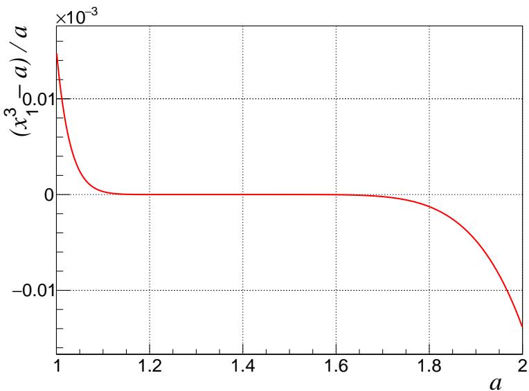
Figure 1. The cubic root error $h_1$ after the first 9th order iteration step starting from $x_0=1.104$.

中

图 1. 从 $x_0=1.104$ 出发、经过第一次九阶迭代步骤后的立方根误差 $h_1$。

1. Rounding Error Analysis

EN

Below is the C code corresponding to the algorithm proposed above, with a cubic minimax polynomial for the initial approximation, a first cubic Newton iteration in double precision, and another classical second-order Newton iteration in double-double precision. Here zz is the input reduced to the range [1, 8), and z is reduced to [1, 2). The constants $c_0,c_1,c_2,c_3$ are those of a minimax polynomial of $x^{1/3}$ over [1, 2], namely (in hexadecimal notation) c[0]=0x1.1b0babccfef9cp-1, c[1]=0x1.2c9a3e94d1da5p-1, c[2]=-0x1.4dc30b1a1ddbap-3, c[3]=0x1.7a8d3e4ec9b07p-6. The value cvt2.f is either 1 when $1\le zz<2$, the approximation 0x1.428a2f98d728bp+0 of $2^{1/3}$ when $2\le zz<4$ or when $4\le zz<8$ the approximation 0x1.965fea53d6e3dp+0 of $2^{2/3}$. All variables have double precision, and we renamed some variables for better clarity:

- r = 1/z
- z2 = z*z
- c0 = c[0]+z*c[1]
- c2 = c[2]+z*c[3]
- y0 = c0 + z2*c2
- y2a = y0*y0

中

下面是对应于上述算法的 C 代码：用一个三次 minimax 多项式做初始近似，第一次立方 Newton 迭代采用双精度，另一次经典的二阶 Newton 迭代采用双倍双精度。这里 zz 是归约到区间 [1, 8) 的输入，z 归约到 [1, 2)。常数 $c_0,c_1,c_2,c_3$ 是 $x^{1/3}$ 在 [1, 2] 上的 minimax 多项式系数，即（十六进制表示）c[0]=0x1.1b0babccfef9cp-1、c[1]=0x1.2c9a3e94d1da5p-1、c[2]=-0x1.4dc30b1a1ddbap-3、c[3]=0x1.7a8d3e4ec9b07p-6。cvt2.f 的取值是：当 $1\le zz<2$ 时为 1；当 $2\le zz<4$ 时为 $2^{1/3}$ 的近似 0x1.428a2f98d728bp+0；当 $4\le zz<8$ 时为 $2^{2/3}$ 的近似 0x1.965fea53d6e3dp+0。所有变量都是双精度，为清晰起见我们对一些变量做了重命名：

- r = 1/z
- z2 = z*z
- c0 = c[0]+z*c[1]
- c2 = c[2]+z*c[3]
- y0 = c0 + z2*c2
- y2a = y0*y0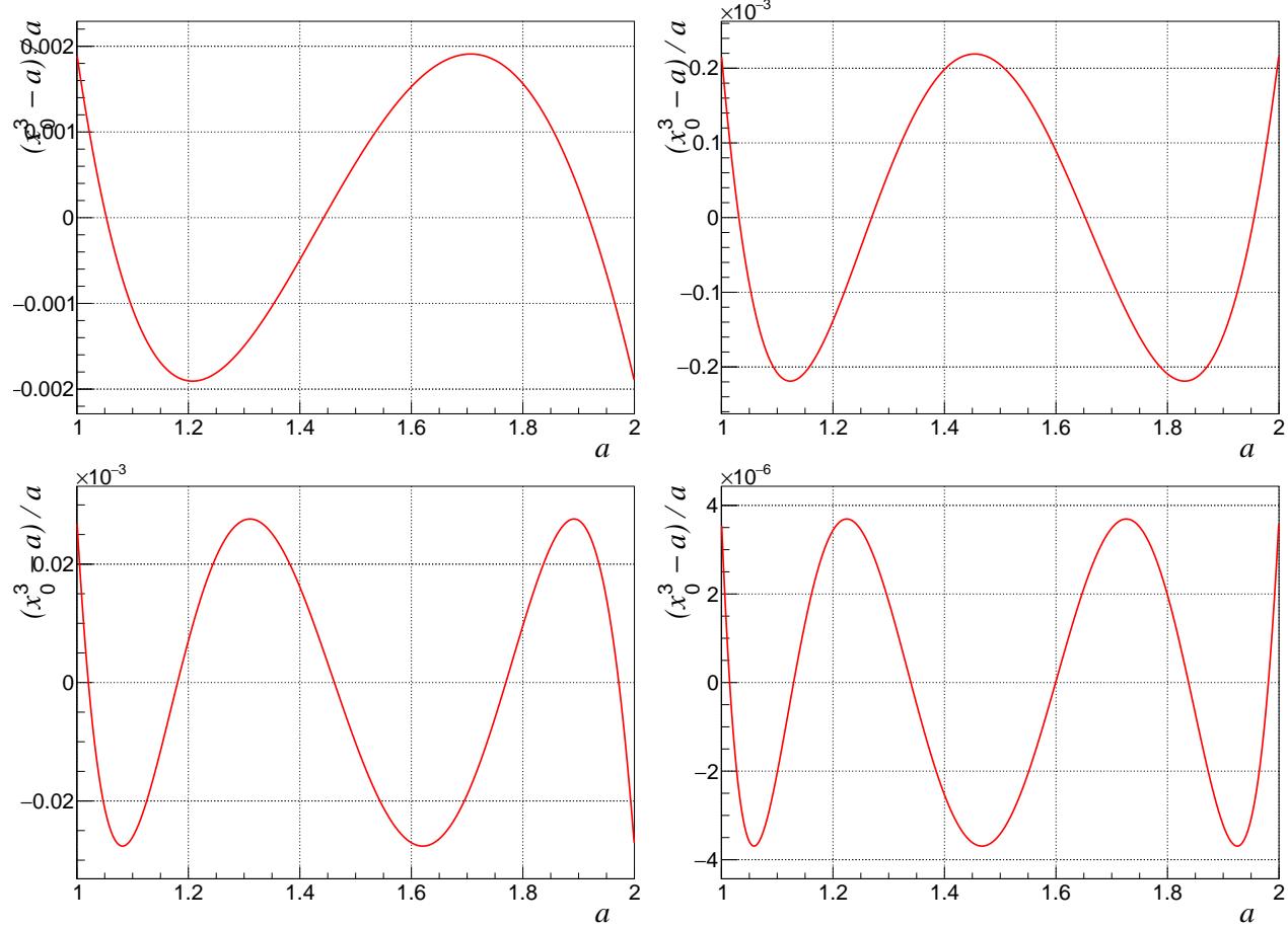

EN

Then the second block of instructions is:

- h0 = y2a*(y0*r) - 1
- y1 = y0 - (h0*y0)*(u0 - u1*h0)
- y1 *= cvt2.f
- y2h = y1*y1
- y2l = fma(y1,y1,-y2h)
- y3 = y2h*y1
- y3l = fma(y1,y2h,-y3) + y1*y2l
- h1 = ((y3 - zz) + y3l)*rr
- dy = h1*(y1*u0)

中

第二段指令为：

- h0 = y2a*(y0*r) - 1
- y1 = y0 - (h0*y0)*(u0 - u1*h0)
- y1 *= cvt2.f
- y2h = y1*y1
- y2l = fma(y1,y1,-y2h)
- y3 = y2h*y1
- y3l = fma(y1,y2h,-y3) + y1*y2l
- h1 = ((y3 - zz) + y3l)*rr
- dy = h1*(y1*u0)

EN

Then y1 - dy is a good approximation of $z{z}^{1/3}$.

If there are no rounding errors, the algorithm corresponds to a rational approximation $p(x)/q(x)$, where $p$ has degree 84 and coefficients up to 569 digits, and $q(x)=k{x}^9$, where $k$ is an integer of 569 digits (in the case $1\le x\le 2$).

中

于是 y1 - dy 就是 $z{z}^{1/3}$ 的一个良好近似。

若不存在舍入误差，该算法对应于一个有理逼近 $p(x)/q(x)$，其中 $p$ 为 84 次多项式、系数最多 569 位，而 $q(x)=k{x}^9$，$k$ 是一个 569 位的整数（在 $1\le x\le 2$ 的情形下）。

EN

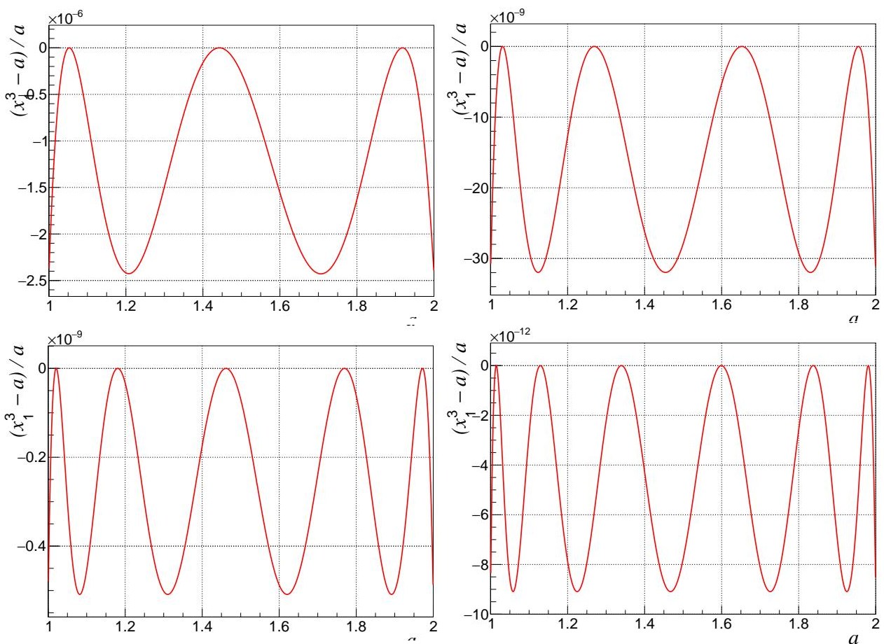
Figure 3. The error $h_1$ after the first second order Newton iteration step for various initial approximations. The plot order is the same as in Fig. 2.

中

图 3. 针对各种初始近似、在第一次二阶 Newton 迭代步骤之后的误差 $h_1$。子图顺序与图 2 相同。

EN

To each floating-point operation which can produce a rounding error, say $a+b$, we associate a variable, say $\delta$, representing the corresponding error. We replace the expression $a+b$ by $a+b+\delta$ in $p(x)/q(x)$, differentiate with respect to $\delta$ and replace $\delta$ by 0. This yields the first-order derivative, say $f(x)$, of the cubic root approximation $p(x)/q(x)$ with respect to the rounding error $\delta$. We then compute the maximal absolute value of $f(x)$ over the whole interval [1, 8]. We call this value the sensitivity with respect to $\delta$, and we denote it by $s$. By the Taylor theorem with explicit remainder, the error in the approximation of $x^{1/3}$ coming from the rounding error in $a+b$ is bounded by $s$ times the maximal value of $\delta$. And for several rounding errors ${\delta }_0,{\delta }_1,\dots$ with sensitivities $s_0,s_1,\dots$, the final error is bounded by $s_{0}max|{\delta }_0|+s_{1}max|{\delta }_1|+\cdots$.

Note: we take into account that the subtraction h = y2*(y*r) - 1 is exact due to Sterbenz' theorem.

中

对于每一个可能产生舍入误差的浮点运算，比如 $a+b$，我们关联一个变量（比如 $\delta$）来表示相应的误差。我们把 $p(x)/q(x)$ 中的表达式 $a+b$ 替换为 $a+b+\delta$，对 $\delta$ 求导，再令 $\delta =0$。这样就得到立方根逼近 $p(x)/q(x)$ 关于舍入误差 $\delta$ 的一阶导数，记为 $f(x)$。然后计算 $f(x)$ 在整个区间 [1, 8] 上的最大绝对值。我们把这个值称为关于 $\delta$ 的灵敏度（sensitivity），记为 $s$。根据带显式余项的 Taylor 定理，由 $a+b$ 中的舍入误差所导致的 $x^{1/3}$ 逼近误差以 $s$ 乘以 $\delta$ 的最大值为界。对于若干个舍入误差 ${\delta }_0,{\delta }_1,\dots$（灵敏度分别为 $s_0,s_1,\dots$），最终误差以 $s_{0}max|{\delta }_0|+s_{1}max|{\delta }_1|+\cdots$ 为界。

注：我们利用了减法 h = y2*(y*r) - 1 由 Sterbenz 定理保证精确这一点。

EN

The two instructions y2h = y1*y1 and y2l = fma(y1, y1, -y2h) compute a double-double approximation y2h + y2l of y1*y1. In the rounding to nearest mode, we have exactly y2h + y2l = y1*y1. For directed rounding modes, since y1*y1 can be represented exactly with 106 bits, we can write y1*y1 = h + l with h being the rounding of y1*y1 towards zero, and l representable in double precision. If y2h = h, then y1*y1 - y2h = l and can be represented exactly, thus y2h + y2l = y1*y1. Now if y2h = nextabove(h), then y1*y1 - y2h = h + l - (h + ulp(h)) = l - ulp(h), and since ulp(l) is larger or equal to ulp(h) multiplied by $2^{-53}$, the difference ulp(h) - l is exactly representable. In summary, for all rounding modes we have y1*y1 = y2h + y2l exactly. Similarly, we have y2h*y1 = y3 + y3l exactly, thus y1*y1*y1 = y3 + y3l + delta17, where delta17 is the rounding error in y1*y2l. Since y1 is less than 2, and y2l is less than ulp(y1*y1) which is $2^{-52}$, y1*y2l is bounded by $2^{-51}$, and the rounding error on y1*y2l is thus $|{\delta }_{17}|\le 2^{-104}$.

中

指令 y2h = y1*y1 和 y2l = fma(y1, y1, -y2h) 计算 y1*y1 的双倍双精度近似 y2h + y2l。在就近舍入模式下，精确地有 y2h + y2l = y1*y1。对于方向舍入模式，由于 y1*y1 可以用 106 位精确表示，我们可以写成 y1*y1 = h + l，其中 h 是 y1*y1 向零舍入的结果，l 可以用双精度表示。若 y2h = h，则 y1*y1 - y2h = l 且能精确表示，因此 y2h + y2l = y1*y1。若 y2h = nextabove(h)，则 y1*y1 - y2h = h + l - (h + ulp(h)) = l - ulp(h)，又由于 ulp(l) 大于等于 ulp(h) 乘以 $2^{-53}$，差 ulp(h) - l 可以精确表示。总之，对所有舍入模式，都精确地有 y1*y1 = y2h + y2l。类似地，精确地有 y2h*y1 = y3 + y3l，因此 y1*y1*y1 = y3 + y3l + delta17，其中 delta17 是 y1*y2l 的舍入误差。由于 y1 小于 2，而 y2l 小于 ulp(y1*y1)（即 $2^{-52}$），y1*y2l 以 $2^{-51}$ 为界，故 y1*y2l 上的舍入误差满足 $|{\delta }_{17}|\le 2^{-104}$。

EN

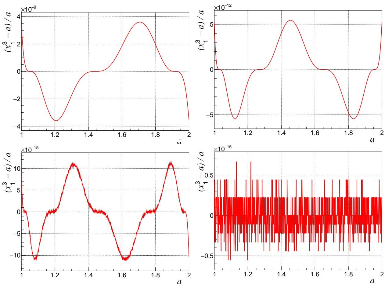
Figure 4. The error $h_1$ after the first third order Newton iteration step for various initial approximations. The plot order is the same as in Fig. 2.

中

图 4. 针对各种初始近似、在第一次三阶 Newton 迭代步骤之后的误差 $h_1$。子图顺序与图 2 相同。

EN

When one adds all rounding error bounds from Table 1, one gets a maximum error (due to roundings) of $1.13\cdot {10}^{-26}$. If we add the $1.13\cdot {10}^{-26}$ bound for the rounding error to the $1.32\cdot {10}^{-23}$ bound for the mathematical error, we get a global bound of $1.322\cdot {10}^{-23}<2^{-76}$ thus we can use $2^{-76}$ as error margin in the rounding test.

中

把表 1 中所有的舍入误差界相加，得到最大误差（由舍入引起）为 $1.13\cdot {10}^{-26}$。把舍入误差的界 $1.13\cdot {10}^{-26}$ 与数学误差的界 $1.32\cdot {10}^{-23}$ 相加，得到全局界 $1.322\cdot {10}^{-23}<2^{-76}$，因此我们可以在舍入测试中使用 $2^{-76}$ 作为误差裕度。

EN

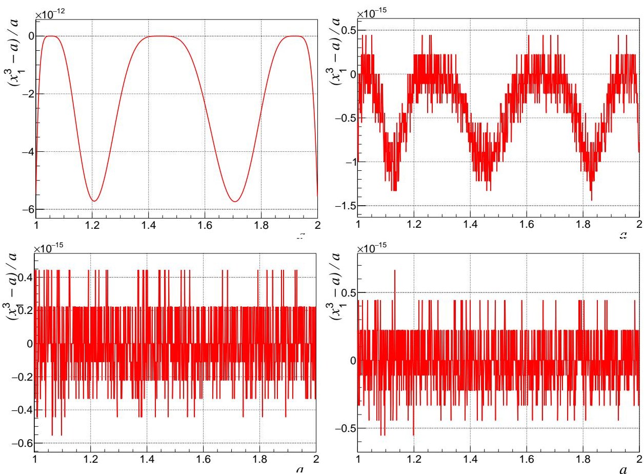
Figure 5. The error $h_1$ after the first quartic order Newton iteration step for various initial approximations. The plot order is the same as in Fig. 2.

中

图 5. 针对各种初始近似、在第一次四阶 Newton 迭代步骤之后的误差 $h_1$。子图顺序与图 2 相同。

References

EN

[1] Boldo, S., Graillat, S., and Muller, J. On the robustness of the 2Sum and Fast2Sum algorithms. ACM Trans. Math. Softw. 44, 1 (2017), 4:1–4:14.

中

[1] Boldo, S., Graillat, S., and Muller, J. On the robustness of the 2Sum and Fast2Sum algorithms. ACM Trans. Math. Softw. 44, 1 (2017), 4:1–4:14。（关于 2Sum 与 Fast2Sum 算法的稳健性。）

Figures 6–10 / 图 6–10

EN

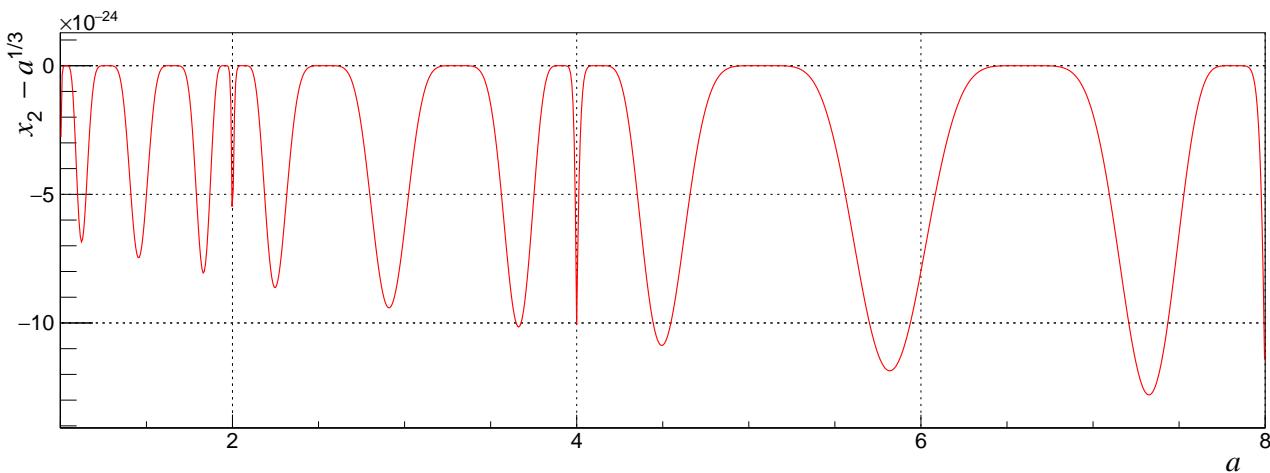
Figure 6. The error of the cubic root evaluation after the refinement step where the root $x_2$ is represented as an unevaluated sum of two numbers in binary64 $x_2=x_2^{\mathrm{high}}+x_2^{\mathrm{low}}$.

中

图 6. 精化步骤之后立方根求值的误差，其中根 $x_2$ 表示为两个 binary64 数的未求和：$x_2=x_2^{\mathrm{high}}+x_2^{\mathrm{low}}$。

EN

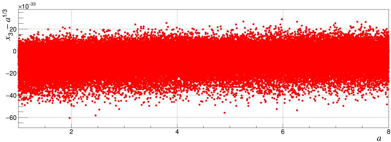
Figure 7. The error of the cubic root evaluation for the worst case when the rounding test fails and the additional Newton iteration step is taken. FPU is operating in the round-to-nearest mode.

中

图 7. 在最坏情形（舍入测试失败、执行额外 Newton 迭代步骤）下立方根求值的误差。FPU 工作在就近舍入模式。

EN

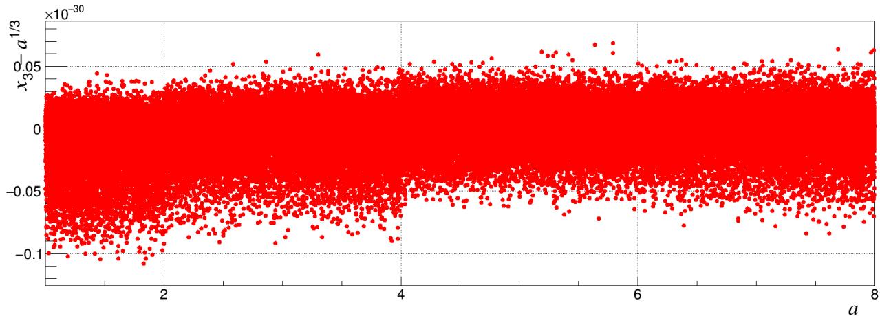
Figure 8. The error of the cubic root evaluation for the worst case when the rounding test fails and the additional Newton iteration step is taken. FPU is operating in the downward mode.

中

图 8. 在最坏情形（舍入测试失败、执行额外 Newton 迭代步骤）下立方根求值的误差。FPU 工作在向下舍入模式。

EN

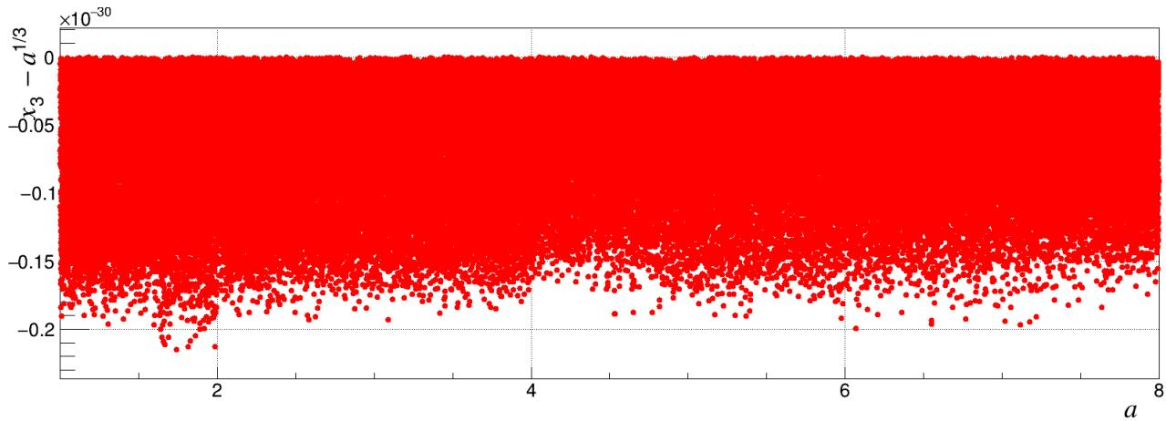
Figure 9. The error of the cubic root evaluation for the worst case when the rounding test fails and the additional Newton iteration step is taken. FPU is operating in the upward mode.

中

图 9. 在最坏情形（舍入测试失败、执行额外 Newton 迭代步骤）下立方根求值的误差。FPU 工作在向上舍入模式。

EN

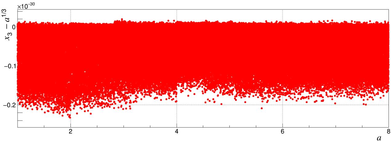
Figure 10. The error of the cubic root evaluation for the worst case when the rounding test fails and the additional Newton iteration step is taken. FPU is operating in the toward-zero mode.

中

图 10. 在最坏情形（舍入测试失败、执行额外 Newton 迭代步骤）下立方根求值的误差。FPU 工作在向零舍入模式。

Table 1

EN

Table 1. The sensitivities $s_i$ and maximal values of ${\delta }_i$ for all rounding errors that can occur in the algorithm.

中

表 1. 算法中可能出现的所有舍入误差所对应的灵敏度 $s_i$ 与 ${\delta }_i$ 的最大值。

${\delta }_i$	instruction	sensitivity $s_i$	$max|{\delta }_i|$	$s_i\cdot max|{\delta }_i|$
${\delta }_0$	r=1/z	$2^{-38.5}$	$2^{-53}$	$2^{-91.5}$
${\delta }_1$	z2 = z*z	$2^{-62.8}$	$2^{-51}$	$2^{-113.8}$
${\delta }_2$	z*c[1]	$2^{-60.0}$	$2^{-52}$	$2^{-112.0}$
${\delta }_3$	c[0]+z*c[1]	$2^{-60.0}$	$2^{-52}$	$2^{-112.0}$
${\delta }_4$	z*c[3]	$2^{-58.0}$	$2^{-57}$	$2^{-115.0}$
${\delta }_5$	c[2]+z*c[3]	$2^{-58.0}$	$2^{-55}$	$2^{-113.0}$
${\delta }_6$	z2*c2	$2^{-60.0}$	$2^{-54}$	$2^{-104.0}$
${\delta }_7$	y0=c0+z2*c2	$2^{-60.0}$	$2^{-52}$	$2^{-102.0}$
${\delta }_8$	y2a=y0*y0	$2^{-37.9}$	$2^{-52}$	$2^{-89.9}$
${\delta }_9$	y0*r	$2^{-36.9}$	$2^{-53}$	$2^{-89.9}$
${\delta }_{10}$	y2a*(y0*r)	$2^{-37.5}$	$2^{-52}$	$2^{-89.5}$
${\delta }_{11}$	h0*y0	$2^{-37.9}$	$2^{-64}$	$2^{-101.9}$
${\delta }_{12}$	u1*h0	$2^{-48.1}$	$2^{-67}$	$2^{-115.1}$
${\delta }_{13}$	u0-u1*h0	$2^{-48.1}$	$2^{-54}$	$2^{-102.1}$
${\delta }_{14}$	(h0*y0)*(u0-u1*h0)	$2^{-36.3}$	$2^{-65}$	$2^{-101.3}$
${\delta }_{15}$	y1=y0-...	$2^{-36.3}$	$2^{-52}$	$2^{-88.3}$
${\delta }_{16}$	y1 *= cvt2.f	$2^{-37.0}$	$2^{-51}$	$2^{-88.0}$
${\delta }_{17}$	error on y1*y1*y1	$2^{-1.5}$	$2^{-104}$	$2^{-105.5}$
${\delta }_{18}$	h1 = ((y3 - zz) + y3l)*rr	$2^{-0.5}$	$2^{-90}$	$2^{-90.5}$
${\delta }_{19}$	y1*u0	$2^{-37.4}$	$2^{-52}$	$2^{-89.4}$
${\delta }_{20}$	h1*(y1*u0)	1	$2^{-91}$	$2^{-91.0}$